When Good Pi Goes Bad

Download the ISF Shaders from this post

As Pi Day approaches this year we've found ourselves Pi-nspired to examine the usage of Pi in some of the more commonly used GLSL generators and FX that people are familiar with and, just for fun, some new shaders that are designed to see what happens when you use a bad estimates for Pi.

What is Pi exactly? If it has been a while since your last geometry class, we've got a very quick explainer for you.

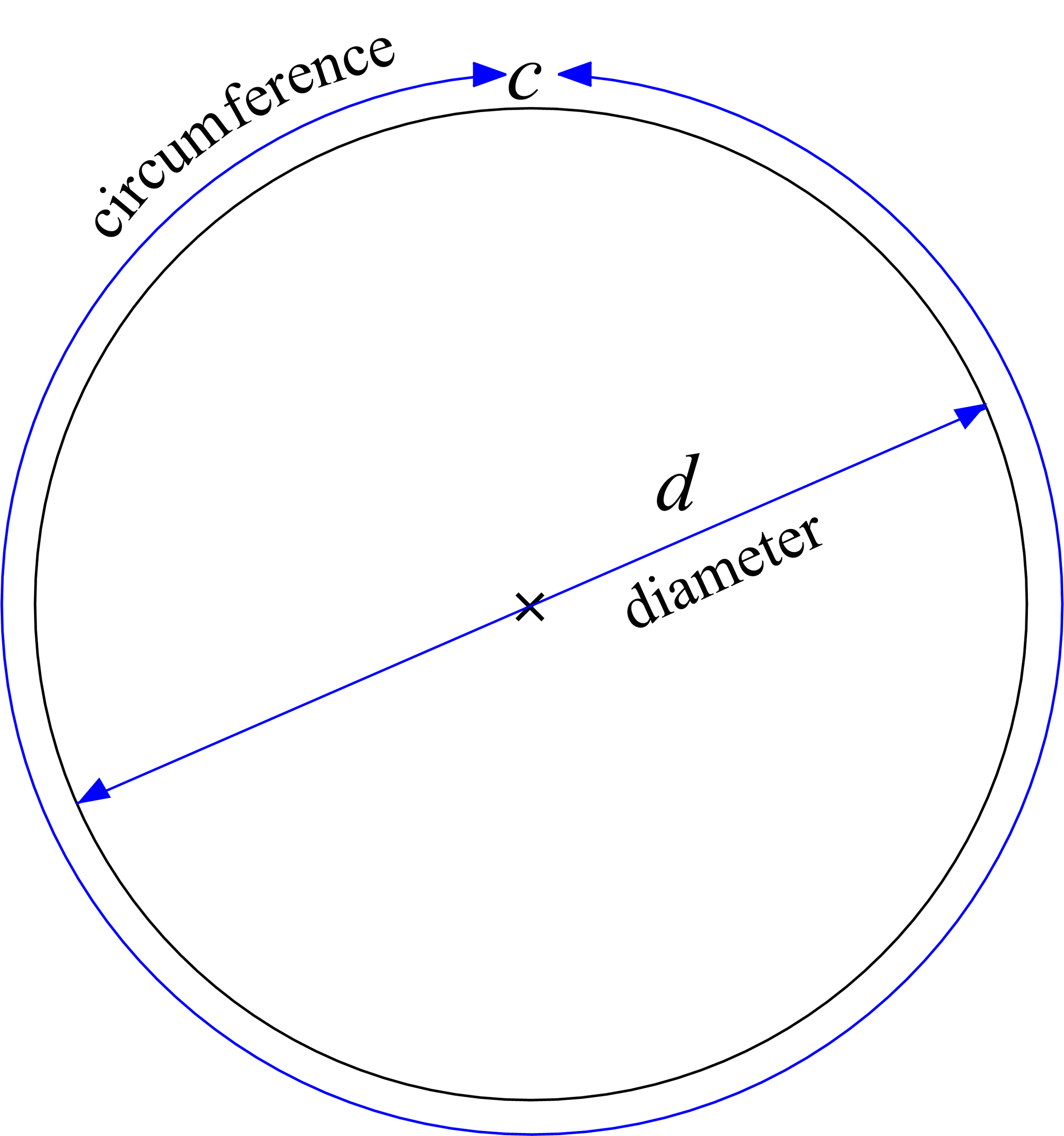
Pi, also written as π (opt-p on your Mac keyboard!) is the number that you get when you have a circle and divide the diameter (the distance from one side of the circle to the other, passing through the center) and the circumference (the distance it takes to travel all the way around the circle). No matter how big or small of a circle, you get the same number, π, when you divide C/d. Sometimes instead of using the diameter this ratio is described by using the distance from the center to any point on the circle, which is called the radius. The radius is always half of the diameter.

The Wikipedia page for Pi has a nice gif that shows this visually, with a circle being rolled out along a ruler.

What makes π a bit tricky to fully understand is that it is what is known in mathematics as as irrational number, which means that it can not be represented by a fraction. When trying to write Pi as a decimal number, it goes on forever. When it comes to performing calculations that rely on Pi, we can only approximate its value. As such, this special number needs its own symbol, π.

π to 100 digits is: 3.1415926535 8979323846 2643383279 5028841971 6939937510 5820974944 5923078164 0628620899 8628034825 3421170679

Since the discovery of π as a numerical constant there have been countless efforts to not just find better approximations of π, but to find algorithms that can calculate those approximations even faster. So, what happens when you have a bad approximation of π, to what degree of accuracy is needed when performing math operations in GLSL, and exactly how long does it take for some of these algorithms to calculate a good approximation of π? These seem like some fun questions to explore by ... writing some shaders!

Before we get into our examples for creating approximations of π, lets take a quick look at a few examples of three very common geometric / distortion filters that make use of it,

• Bump Distortion: Converts the pixel xy to polar coordinates, adjusts the radius, and then reverses back to the Cartesian coordinate system to read the source pixel.

• Rotate: Converts to polar coordinates, adjusts angle, then back to Cartesian coordinates

• Twirl: Converts to polar coordinates, adjusts the radius and angle, and then back to Cartesian coordinates

π is also often used for shaders that draw curves that make use of trigonometric functions like sine and cosine.

We can also visualize how having a bad estimate of Pi can throw off calculations and comparing them to a good known estimate of Pi. One way of doing this is by computing cosine curves using our estimates and observing how the error compounds as the input value increases.

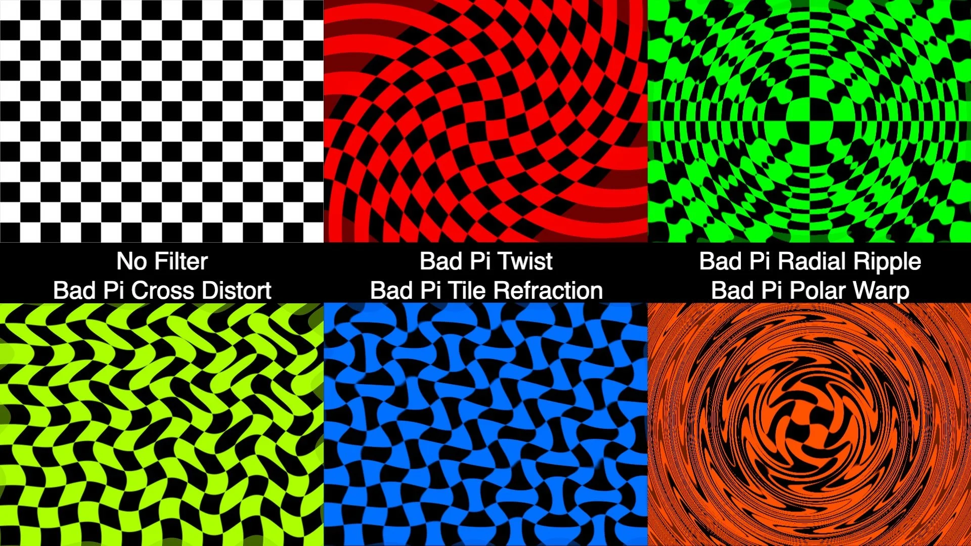
In the set of "Bad Pi.fs" examples we have a few demonstrations of shaders that generate various shapes and patterns using both π and a bad approximation of π. The amount of error added / subtracted can be adjusted using the 'pierror' input for these ISFs. The default range for the 'pierror' input is +/- 0.25, but you can go and edit these values to experiment with seeing what happens with even more error.

The 'Bad Pi Checkerboard.fs' makes its pattern by thresholding sin(x pi gridSize) sin(y pi * gridSize) and makes for a particularly good visualizer with high values for the gridSize. In this video we can see the pi error moving from -0.25 to 0.25 with a gridSize of 24.

While these are some pretty basic demonstrations, the concept of having waveforms and patterns that are out of phase in interesting ways can be extremely powerful when making shaders that have semi-random behaviors. For starters, check out the "Bad Pi FX" examples which create various forms of distortions by using the difference between using good and bad π values in our shaders. When no error is added to π, these filters work as a simple pass through.

Now that we have an idea of what happens when π goes bad, let’s take a look at some of the ways that π itself can be estimated and how look it takes. Of course in typical usage for GLSL shaders, π is usually pre-defined as a fixed constant to at least 10 or 11 decimal places.

While there are several different approaches to estimating Pi, for this set of examples we will be using a method known as Alternating Series.

An alternating series is a summation which switches between adding and subtracting numbers on each iteration. As you approach a very large number of iterations some alternating series will eventually begin to converge around a fixed number. In some even more special cases, as you take a 'limit' towards an infinite number of iterations, the series may actually reach the value it is converging around.

For example, the infinite geometric series ⁠1/2⁠ − ⁠1/4⁠ + ⁠1/8⁠ − ⁠1/16⁠ + ⋯ eventually sums to ⁠1/3⁠.

The “Estimate Pi.fs” shader demonstrates how Pi can be recursively computed using alternating series, and how the design of the series can greatly change how quickly the series converges. Here we are comparing the Leibniz and the Nilakantha series for π. These are not the only two, there are other approaches, some of which converge even faster.

float estimatePiAdjustmentLeibniz(int n)	{
    float	floatN = float(n);
    float	adjustment = 4.0 / (2.0 * floatN + 1.0);
    //	flip the sign if needed
    adjustment = (mod(floatN,2.0) == 1.0) ? -1.0 * adjustment : adjustment;
    return adjustment;
}

float estimatePiAdjustmentNilakantha(int n)	{
    if (n == 0)	{
        return 3.0;
    }
    //	start this with an index of 1
    float	nPlusOne = float(n + 1);
    float	baseVal = 2.0 * nPlusOne;
    float	adjustment = 4.0 / (baseVal * (baseVal - 1.0) * (baseVal - 2.0));
    //	flip the sign if needed
    adjustment = (mod(nPlusOne,2.0) == 1.0) ? -1.0 * adjustment : adjustment;
    return adjustment;
}

In this case we can see that the Nilakantha for approximating Pi is significantly faster than the Leibniz series. This shader works be performing one iteration each time a new frame is rendered and then uses a second render pass to visualize the current estimates in the style of a seven segment display. The top line shows the Nilakantha approach and the middle line shows the Leibniz value at the same number of iterations.

Running the shader, we can see that the Nilakantha approach converges to 3.14159 very quickly, taking only about 42 iterations (less than a second and a half at 30 fps). By comparison, at this same point the Leibniz is still only at a single decimal point of accuracy. We would have to run the Leibniz for over 5000 iterations (over two and a half minutes at 30 fps) before it even starts to approach four decimal places of accuracy. It would take over an hour to reach 3.14159xxx, somewhere around 137500 iterations.

For its visualization stage the Estimate Pi.fs shader uses a technique for drawing numbers demonstrated in the Digital Clock.fs example.

Combining our initial visualizers with the "Estimate Pi.fs" example we can create a more complex demonstration, such as the 'Bad Pi Visualizer.fs' example included in this download, and render out a few variations to watch, or use as part of a live performance.

You might be asking yourself at this point – why do these estimations iteratively in GLSL? Surely there are better ways for doing this! And you'd be right, we are doing this for fun, for the challenge, and to inspire people to come up with their own variations on this idea.

Side note: The Estimate Pi and Bad Pi Visualizer shaders make use of 32-bit floating point textures for an intermediate render pass, unfortunately this means they only work in hosts that support 32-bit floating point texture ISF render passes. This means they do not work with the current web based version of ISF shader, so you'll need to download them to try them out for yourself.

Some more related links:
https://en.wikipedia.org/wiki/Leibniz_formula_for_π
https://observablehq.com/@galopin/an-infinite-series-that-converges-quickly-on-pi
https://www.tylar.io/programs/finished/piCalculator/index.html
https://editor.p5js.org/codingtrain/sketches/8nvCqk0-W

Some techniques for drawing text in GLSL

Download the example ISF compositions from this tutorial.

View fullsize

Rendering TG Character Test.fs in the ISF Editor utility.

While GLSL is not a particularly great language for rendering text strings, many shader developers have found it a fun challenge to do so anyway. Over the years we’ve run into several interesting blog posts and examples from people showing off different techniques that they’ve come up with. In this write up we are going to look at three ‘common’ approaches to drawing text in GLSL along with how the concepts can be adapted when making ISF shaders:

• Using a bitmap image of characters as a lookup.

• Encoding the bytes from a bitmap font in an array as part of the shader.

• Individually drawing each character in GLSL.

As with most coding problems even within these general techniques there are several ways the objective can be solved, and no doubt other clever developers out there will continue to come up with other approaches that will leave our mouths agape.

---

Rendering text in GLSL using fonts encoded in bitmap images

The first technique we will look at is very well covered in the blog post Text Rendering by Jon Baker. describes how a monospaced font can be encoded into a bitmap image which is read from as part of the shader: “we're using a bitmapped monospaced font, where every font glyph is 6 pixels wide and 8 pixels tall.”

Within the shader itself each “cell” can determine its own local pixel coordinates and then look up the corresponding pixel from the provided bitmap image for the desired ASCII character to display.

ISF allows us to include images and reference them in the JSON blob, which you can find in the top portion of the JB Monospace Character Test.fs example.

/*{
    "CATEGORIES": [
        "Text"
    ],
    "CREDIT": "Jon Baker, adapted by VIDVOX",
    "IMPORTED": {
        "fontImage": {
            "PATH": "jbakermonospaced.png"
        }
    },
     "DESCRIPTION": "Test for drawing characters from a bitmap font stored as an image.",
    "INPUTS": [
 ...
    ],
    "ISFVSN": "2"
}
*/

View fullsize

The bitmap image containing the font.

This basic test shader provides us with a slider (float) with a range of 0 to 255 for selecting which character we want to repeat in each cell. It also includes a toggle button (boolean) for enabling the debug mode for visualizing the local pixel coordinates for each cell. When loaded into a host app like VDMX, it looks like this:

View fullsize

Rendering JB Monospace Character Test.fs in VDMX6 with the debugOverlay enabled to show the local pixel coordinates for each cell.

Building on the test shader we can create something more complex, such as the JB Monospace Random Characters.fs example which renders an image full of random characters each with a random color. For this ISF the debug option has been extended to show either the local coordinates for each cell or the coordinates of each cell within the whole grid.

View fullsize

Rendering JB Monospace Random Characters.fs in VDMX. Includes sliders for adjusting the random seeds of the characters independently from the hues.

---

Encoding the bytes from a bitmap font in an array as part of the shader

The character A encoded in 16 bytes, stored as an uvec4, that’s 4 uints with each 4 bytes, from Texture-less Text Rendering.

Another approach that is well documented involves taking the data from a bitmap font file and encoding the byte values directly into the shader as an array. Here we are going to mainly look at two blog posts:

• Tim Gfrerer’s wonderful post Texture-less Text Rendering uses the PSF1 and an in depth explanation of their implementation as a GLSL shader.

• Jon Baker has made a beautiful adaptation of Code page 437, an extended ASCII table which shipped with the IBM PC, written as a GLSL shader. In the blog post Siren: Masks Planes he details the process of how he came up with and implemented the idea.

The Texture-less Text Rendering approach described by Tim has four steps:

1. Get the bitmap data from the font file.

2. Embed the byte data as an array in the shader file.

3. Use another array to hold the character code values for a word.

4. Looking up the character data for each index in the word array.

View fullsize

Using the ISF Editor to translate syntax between variations of GLSL.

While ISF allows for a custom vertex shader, to keep things simple for future remixing, for the TG Character Test.fs adaptation we put everything in the fragment shader. Starting from the debug_text.frag in the GitHub repository referenced in the blog post, there were a number of minor syntax changes that were needed to adapt this for ISF. Fortunately they were all fairly easy to handle by hand using the error messages in the ISF Editor utility.

Like with the basic test shader using the bitmap lookup, before getting into Tim’s approach for displaying full words and phrases, it is useful to start with an example that just generates a display for every possible character, along with the ability to test displaying a specific character. This makes it easy to verify each part of the shader is working as expected and validate the drawing.

With this working, creating an extra constant to hold the full phrase for display and swapping it out for our debug code, we now have a full implementation of Tim’s technique in TG Message Test.fs. This trick for holding a phrase as character codes in an array can also be used along with the bitmap image approach above.

We won’t go into converting it to ISF, but a third example of this approach can be found in the debugtext.comp.glsl shader from the niagara project.

View fullsize

View fullsize

View fullsize

Code page 437 font.

Jon Baker uses a similar approach for adapting the Code page 437 font to use a single fragment shader. The blog post diving into how it was developed includes example code shared on ShaderToy. Converting this to ISF is a fun exercise. The big detail is that when using this in VDMX6, the ‘char’ variable is a restricted name by Metal, so we have to change that to something else. Fortunately the error log points this out for us when we try to load it. The adapted shader, JB Code Page 437 Character Test.fs, is set up to just repeat the same character in each cell.

View fullsize

JB Code Page 437 Character Test.fs loaded in VDMX.

---

Drawing individual characters with GLSL code

Perhaps the most tedious version approach that we will look at in this discussion is using code to render out specific characters that are needed. Two examples of this are included in the standard set of ISF shaders:

• Digital Clock.fs

• ASCII Art.fs

In Digital Clock.fs, only the digits 0-9 and a colon are needed for display, so while this can be time consuming to write, there are only a handful of cases to deal with. The functions found in this example can be very useful in situations where only numbers are appropriate to be rendered.

View fullsize

Function for drawing a digit in Digital Clock.fs.

View fullsize

Rendering Digital Clock.fs in VDMX with the Bad TV effect added.

In ASCII Art.fs, the code for each character rendered was created by movAX13h using a custom tool to generate the code snippets for the supported characters: “: * o & 8 @ #” – while this is not useful for general purpose text writing, it works great in this use case where only a few are needed to match up with different brightness levels.

Another example of this approach in action can be found in the Text with Truchets Demo on ShaderToy.

---

Why convert these to ISF?

ISF (the Interactive Shader Format) is a useful standard for creating ‘write once’ shaders that can be used across different host applications as generators and filters. It allows for playing with and remixing GLSL based compositions without the extra effort of having to build an environment for rendering shaders and all the related code to get a basic pipeline running.

---

Other approaches…

These are of course not the only ways to go about drawing text in GLSL, for example Jazz Mickle has a great post describing their bitmap font renderer for Unity that is worth reading. If you have seen any others that we should check out, please send us an email with a link!